Reading instances and parity with PyVRP

library(vrpr)

Standard instance formats

vrpr ships native readers for the two most common benchmark formats, with no Python dependency. Both return a vrpr_model you can solve right away.

VRPLIB / TSPLIB

read_vrplib() reads CVRP (and VRPTW) instances in the VRPLIB/CVRPLIB format – for example the well-known X set of Uchoa et al. It supports Euclidean coordinates (EDGE_WEIGHT_TYPE : EUC_2D) and reads time-window and service-time sections when present.

path <- system.file("extdata", "sample-n6-k2.vrp", package = "vrpr")

model <- read_vrplib(path)
#> ✔ Read "sample-n6-k2": 5 clients, 1 depot, capacity 30, 2 vehicles.
model
#> 
#> ── VRP model ───────────────────────────────────────────────────────────────────
#> • 1 depot
#> • 5 clients
#> • 1 vehicle type

res <- vrp_solve(model, stop = max_iterations(300), seed = 1, display = FALSE)
plot(res)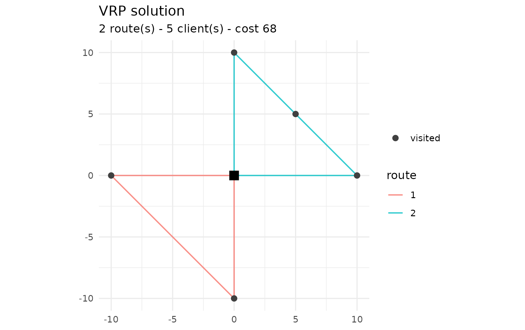

The number of vehicles is taken from the VEHICLES/TRUCKS field, or from the -k<n> suffix in the instance name, or — as a last resort — the number of clients. You can always override it with num_vehicles =.

Solomon

read_solomon() reads VRPTW instances in the Solomon (and Gehring-Homberger) format: a VEHICLE section with the fleet size and capacity, and a CUSTOMER table with coordinates, demand, time window and service time. Customer 0 is the depot.

path <- system.file("extdata", "sample-solomon.txt", package = "vrpr")
read_solomon(path) |>
  vrp_solve(stop = max_iterations(300), seed = 1, display = FALSE) |>
  cost()
#> ✔ Read "SAMPLE": 4 clients, capacity 50, 3 vehicles (VRPTW).
#> [1] 62

Distances

When you do not supply explicit matrices, vrpr computes the Euclidean distance between coordinates and rounds it half up (floor(d + 0.5)) — the TSPLIB EUC_2D convention, which is what the published best-known solutions assume. You can pass your own distance and duration matrices to vrp_problem_data() (and hence to vrp_solve()) for road networks or asymmetric travel times.

Parity with PyVRP

Because vrpr vendors PyVRP’s C++ core, it is faithful to the reference solver on two levels.

Objective parity (exact). The same solution scores identically on both sides, since they share the same C++ CostEvaluator. On the bundled sample-n6-k2 instance, the routes [[1, 2], [3, 4, 5]] cost 81 in both vrpr and PyVRP.

Quality parity. On the X-n101-k25 instance (100 clients, known optimum 27591), a 10-second release build of vrpr reaches the optimum, matching PyVRP, with a comparable number of iterations. The reproducible benchmark lives in tools/benchmark/ (parity.R drives vrpr, pyvrp_side.py the reference).

Solver	cost	gap to optimum
PyVRP	27591	0.00 %
vrpr	27591	0.00 %

When benchmarking, always measure a release build (R CMD INSTALL), not the debug build of devtools::load_all(): the debug build compiles without optimisation and with the core’s assertions enabled, making it many times slower and distorting any throughput comparison.

The algorithm

vrpr runs the same iterated local search as PyVRP: an initial descent, then repeated rounds of perturbation and local search, with Late Acceptance Hill-Climbing (Burke & Bykov, 2017) as the acceptance criterion, a restart from the best after a stretch without improvement, and an exhaustive refinement of each new best. Penalty weights for load, time-window and distance violations are adapted online. Tune any of this through [ils_params()].