A model that fits the past well can still forecast badly.
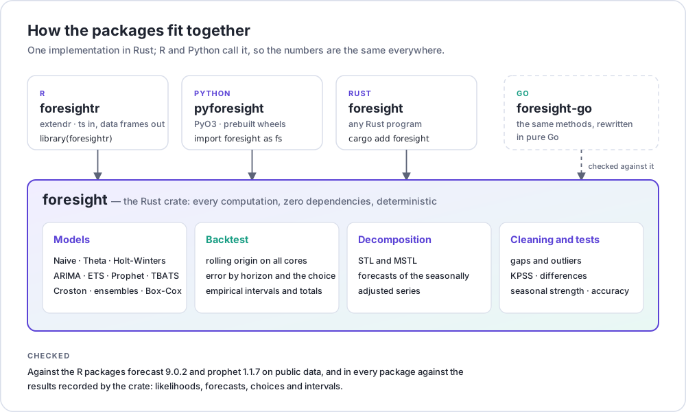
foresightr chooses models the other way round: it replays
the past, and at each point forecasts with what was known then.
The data
Monthly ICMS, the main tax revenue of the Brazilian state of Piauí, from the public fiscal reports (Siconfi/STN). The first observation is March 2017.
path <- system.file("extdata", "piaui_revenue.csv", package = "foresightr")
data <- read.csv(path, comment.char = "#")
# BRL million, monthly from March 2017
icms <- ts(data$icms / 1e6, start = c(2017, 3), frequency = 12)
Choose a model by what would have worked
backtest() refits every candidate at each of the last 36
months, using only the data before it, and forecasts up to 12 months
ahead. The candidates are ranked by their mean absolute percentage
error, the average of the best two is added as one more candidate, and
the best of all forecasts from the whole series.
bt <- backtest(icms)
bt
#> <foresight backtest> 12 candidates, 36 origins, 12 periods ahead
#> Chosen: mean(log_arima_011_011+arima_011_011) (MAPE 3.427)
#>
#>                                     name score
#> 1  mean(log_arima_011_011+arima_011_011) 3.427
#> 2                      log_arima_011_011 3.654
#> 3                          arima_011_011 3.868
#> 4                            log_prophet 4.749
#> 5                                prophet 5.508
#> 6                             log_linear 5.538
#> 7                           holt_winters 7.293
#> 8                                  theta 7.502
#> 9                                  drift 7.857
#> 10                                 naive 8.548
#> ... and 2 more
The forecast of the chosen candidate, with intervals that are quantiles of the errors it made in the backtest, horizon by horizon:
head(bt$forecast)
#> # A tibble: 6 × 7
#>   horizon time        mean lower_80 upper_80 lower_95 upper_95
#>     <int> <date>     <dbl>    <dbl>    <dbl>    <dbl>    <dbl>
#> 1       1 2026-07-01  809.     770.     852.     737.     867.
#> 2       2 2026-08-01  820.     771.     879.     762.     894.
#> 3       3 2026-09-01  824.     786.     881.     779.     894.
#> 4       4 2026-10-01  847.     802.     908.     793.     920.
#> 5       5 2026-11-01  846.     812.     894.     786.     925.
#> 6       6 2026-12-01  875.     831.     930.     815.     939.
autoplot(bt)
#> Warning: Removed 12 rows containing missing values or values outside the scale range
#> (`geom_line()`).
#> `geom_line()`: Each group consists of only one observation.
#> ℹ Do you need to adjust the group aesthetic?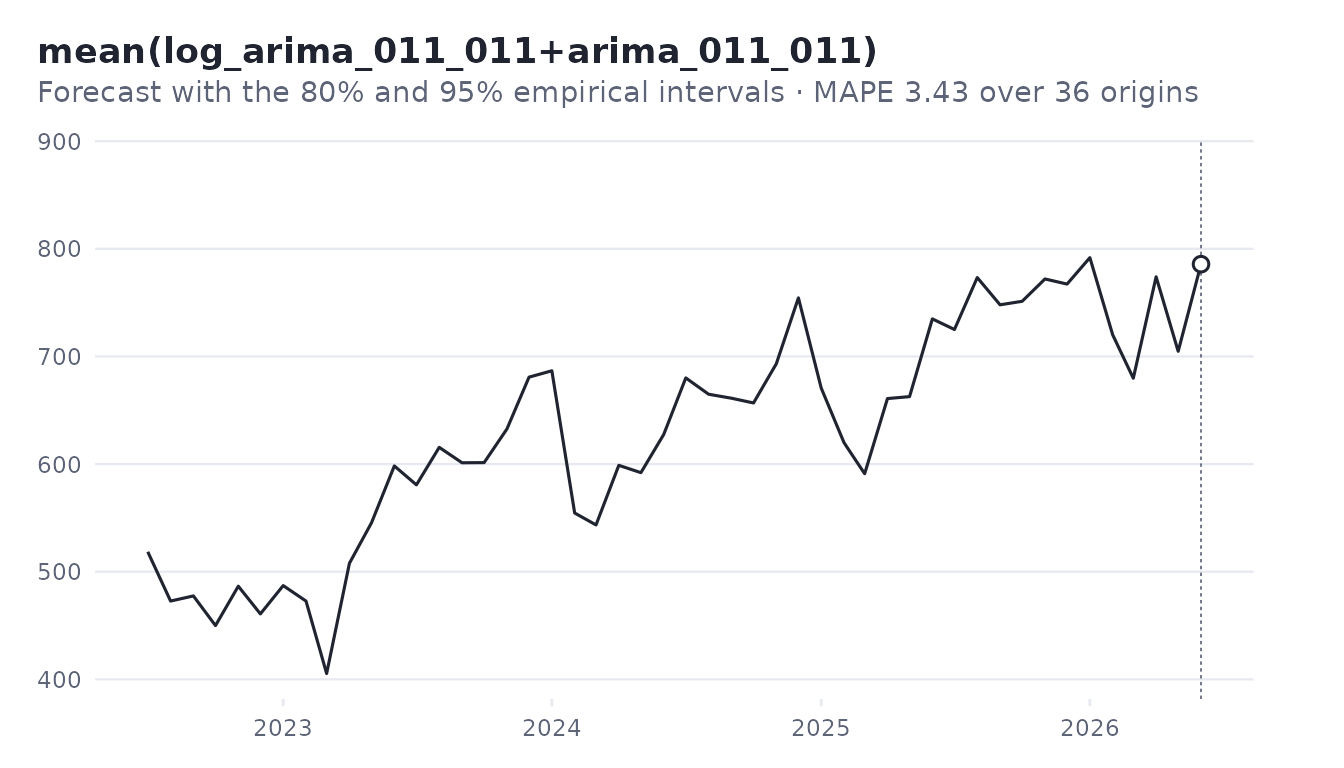
The error of each candidate by horizon:
head(bt$candidates[[bt$best]]$accuracy)
#> # A tibble: 6 × 7
#>   horizon     n  mape   bias   mae  rmse  mase
#>     <int> <dbl> <dbl>  <dbl> <dbl> <dbl> <dbl>
#> 1       1    36  3.53 -0.181  23.8  28.6 0.367
#> 2       2    35  3.61 -0.374  24.2  30.6 0.374
#> 3       3    34  3.54 -0.492  24.1  29.6 0.372
#> 4       4    33  3.31 -0.692  23.1  29.9 0.358
#> 5       5    32  3.42 -1.01   23.8  29.9 0.368
#> 6       6    31  3.63 -1.03   25.1  31.0 0.390
Totals
The total of the next six months has its own interval, measured on totals in the backtest. Adding up the monthly limits would give a wider and wrong interval, because the errors of successive months partly cancel.
total_forecast(bt, 6)
#> # A tibble: 1 × 6
#>   periods  mean lower_80 upper_80 lower_95 upper_95
#>     <int> <dbl>    <dbl>    <dbl>    <dbl>    <dbl>
#> 1       6 5021.    4880.    5248.    4867.    5339.
One model on its own
fit <- fit_model(model_auto_arima(), log(icms))
fit$details$order
#> [1] 0 1 1
fit$details$seasonal_order
#> [1] 0 0 2
exp(predict(fit, 6))
#>           Jul      Aug      Sep      Oct      Nov      Dec
#> 2026 774.9555 782.2726 777.0182 777.1299 784.6480 788.9186
Your own candidates
Any list of models works, renamed as you like; ensembles learn their weights again at every origin of the backtest.
mine <- list(
  with_name(model_seasonal_naive(), "same_month"),
  model_log(model_airline()),
  model_ensemble(candidates_default(), weighting = "stacked")
)
backtest(icms, mine, origins = 24, horizon = 6)$ranking[, c("name", "score")]
#> # A tibble: 4 × 2
#>   name                                     score
#>   <chr>                                    <dbl>
#> 1 same_month                                9.93
#> 2 log_arima_011_011                         4.29
#> 3 ensemble_stacked                          3.88
#> 4 mean(ensemble_stacked+log_arima_011_011)  3.64
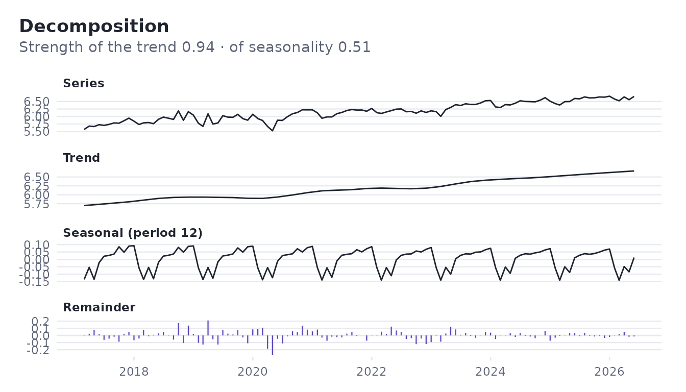
Decomposition
d <- decompose_stl(log(icms), seasonal_window = 13)
d
#> <foresight decomposition> 112 observations, period 12
#> Strength of the trend: 0.939
#> Strength of seasonality (12): 0.515
autoplot(d)