Decomposition and cleaning • foresightr

library(foresightr)

STL

decompose_stl() splits a series into trend, seasonal pattern and remainder by LOESS. Its defaults are those of stats::stl() and, without robust, so are its numbers.

d <- decompose_stl(log(AirPassengers), seasonal_window = 13)
d
#> <foresight decomposition> 144 observations, period 12
#> Strength of the trend: 0.996
#> Strength of seasonality (12): 0.961
autoplot(d)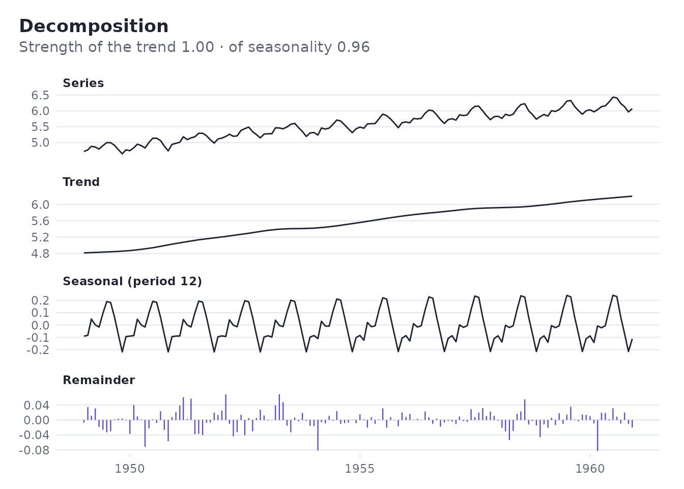

The strengths, from 0 to 1, say how much of the variation the trend and the seasonal pattern explain; seasonal_strength() computes the latter directly. robust = TRUE down-weights outliers.

Several seasonal periods

Daily data often has a weekly and a monthly pattern. decompose_mstl() estimates each in turn:

t <- 0:419
weekly <- c(5, 0, -2, -3, 0, 1, -1)
daily <- 100 + 0.05 * t + weekly[t %% 7 + 1] + 8 * sin(2 * pi * t / 30) +
  2 * sin(t * 1.7) * cos(t * 0.3)
d <- decompose_mstl(daily, periods = c(7, 30))
d$seasonal_strength
#>  seasonal_7 seasonal_30 
#>   0.8464823   0.9687255
autoplot(d)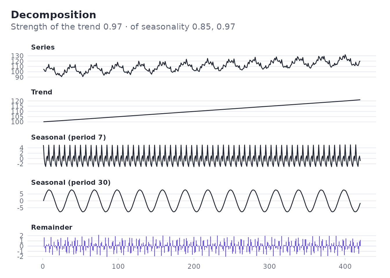

The same decomposition serves to forecast: model_decomposed() runs any model on the seasonally adjusted series and adds the patterns back.

model <- model_decomposed(model_drift(), periods = c(7, 30))
f <- forecast_model(model, daily, 14, period = 7)
round(f, 1)
#>  [1] 127.5 124.1 123.6 124.2 128.3 130.4 129.4 135.8 130.5 128.3 126.9 128.7
#> [13] 128.5 125.4

Gaps and outliers

y <- log(AirPassengers)
y[30] <- y[30] + 0.8     # a typing error
y[100] <- y[100] - 0.7   # a strike
y[61:62] <- NA           # months never recorded
find_outliers(y)
#> # A tibble: 4 × 4
#>   index time       value replacement
#>   <int> <date>     <dbl>       <dbl>
#> 1    30 1951-06-01  5.98        5.22
#> 2    52 1953-04-01  5.46        5.43
#> 3   100 1957-04-01  5.15        5.86
#> 4   135 1960-03-01  6.04        6.15

fill_gaps() fills the missing values following the seasonal pattern; clean_series() also replaces the outliers:

cleaned <- clean_series(y)
round(exp(cbind(dirty = y, clean = cleaned)[c(30, 61, 62, 100), ]))
#>      dirty clean
#> [1,]   396   184
#> [2,]    NA   207
#> [3,]    NA   199
#> [4,]   173   349

Models require complete series, so cleaning comes first when data has gaps. Whether an outlier should be replaced is a judgement about the data: a strike really happened, and removing it may hide a risk that could happen again.