
Introduction
This vignette walks through a realistic analysis using ibger: downloading IPCA (Índice Nacional de Preços ao Consumidor Amplo) inflation data and preparing it for visualization and reporting.
IPCA is Brazil’s official consumer price index, calculated monthly by IBGE. The data is available through aggregate 7060.
Step 1 — Explore the aggregate
Key information from the metadata:
- Periodicity: monthly, from 202001 onwards
- Geographic levels: N1 (Brazil), N6 (municipality), N7 (metropolitan area)
- Variables: monthly change (63), year-to-date (69), 12-month cumulative (2265), and monthly weight (66)
- Classification 315: product groups — 365 categories organized in a hierarchy from the general index down to individual items
# See what variables are available
meta$variables
#> # A tibble: 4 × 3
#>   id    name                                  unit
#>   <chr> <chr>                                 <chr>
#> 1 63    IPCA - Variação mensal                %
#> 2 69    IPCA - Variação acumulada no ano      %
#> 3 2265  IPCA - Variação acumulada em 12 meses %
#> 4 66    IPCA - Peso mensal                    %

# Peek at the classification categories
tidyr::unnest(meta$classifications, categories) |>
  head(20)
#> # A tibble: 20 × 6
#>    id    name             category_id category_name category_unit category_level
#>    <chr> <chr>            <chr>       <chr>         <chr>         <chr>
#>  1 315   Geral, grupo, s… 7169        Índice geral  <NA>          0
#>  2 315   Geral, grupo, s… 7170        1.Alimentaçã… <NA>          1
#>  3 315   Geral, grupo, s… 7171        11.Alimentaç… <NA>          2
#>  4 315   Geral, grupo, s… 7172        1101.Cereais… <NA>          3
#>  5 315   Geral, grupo, s… 7173        1101002.Arroz <NA>          4
#>  6 315   Geral, grupo, s… 7175        1101051.Feij… <NA>          4
#>  7 315   Geral, grupo, s… 7176        1101052.Feij… <NA>          4
#>  8 315   Geral, grupo, s… 47617       1101053.Feij… <NA>          4
#>  9 315   Geral, grupo, s… 12222       1101073.Feij… <NA>          4
#> 10 315   Geral, grupo, s… 47618       1101079.Milh… <NA>          4
#> 11 315   Geral, grupo, s… 7184        1102.Farinha… <NA>          3
#> 12 315   Geral, grupo, s… 7185        1102001.Fari… <NA>          4
#> 13 315   Geral, grupo, s… 7187        1102006.Maca… <NA>          4
#> 14 315   Geral, grupo, s… 7188        1102008.Fubá… <NA>          4
#> 15 315   Geral, grupo, s… 7190        1102010.Floc… <NA>          4
#> 16 315   Geral, grupo, s… 7191        1102012.Fari… <NA>          4
#> 17 315   Geral, grupo, s… 7195        1102023.Fari… <NA>          4
#> 18 315   Geral, grupo, s… 107608      1102029.Mass… <NA>          4
#> 19 315   Geral, grupo, s… 47619       1102061.Maca… <NA>          4
#> 20 315   Geral, grupo, s… 7200        1103.Tubércu… <NA>          3
Step 2 — Monthly IPCA for Brazil
Let’s get the monthly variation for the last 24 months:
ipca_br <- ibge_variables(
  aggregate  = 7060,
  variable   = 63,
  periods    = -24,
  localities = "BR"
)

ipca_br
#> # A tibble: 24 × 9
#>    variable_id variable_name        variable_unit classification_315 locality_id
#>    <chr>       <chr>                <chr>         <chr>              <chr>
#>  1 63          IPCA - Variação men… %             Índice geral       1
#>  2 63          IPCA - Variação men… %             Índice geral       1
#>  3 63          IPCA - Variação men… %             Índice geral       1
#>  4 63          IPCA - Variação men… %             Índice geral       1
#>  5 63          IPCA - Variação men… %             Índice geral       1
#>  6 63          IPCA - Variação men… %             Índice geral       1
#>  7 63          IPCA - Variação men… %             Índice geral       1
#>  8 63          IPCA - Variação men… %             Índice geral       1
#>  9 63          IPCA - Variação men… %             Índice geral       1
#> 10 63          IPCA - Variação men… %             Índice geral       1
#> # ℹ 14 more rows
#> # ℹ 4 more variables: locality_name <chr>, locality_level <chr>, period <chr>,
#> #   value <chr>
The value column is character because of the API’s
special values (see ?parse_ibge_value). Use
parse_ibge_value() to convert:
ipca_br <- ipca_br |>
  mutate(
    value = parse_ibge_value(value),
    date  = as.Date(paste0(period, "01"), format = "%Y%m%d")
  )
Plot the monthly variation
ggplot(ipca_br, aes(date, value)) +
  geom_col(fill = "#2e86c1", alpha = 0.8) +
  geom_hline(yintercept = 0, linewidth = 0.3) +
  labs(
    title    = "IPCA — Monthly variation (%)",
    subtitle = "Brazil, last 24 months",
    x = NULL, y = "Variation (%)",
    caption  = "Source: IBGE via ibger"
  ) +
  theme_minimal()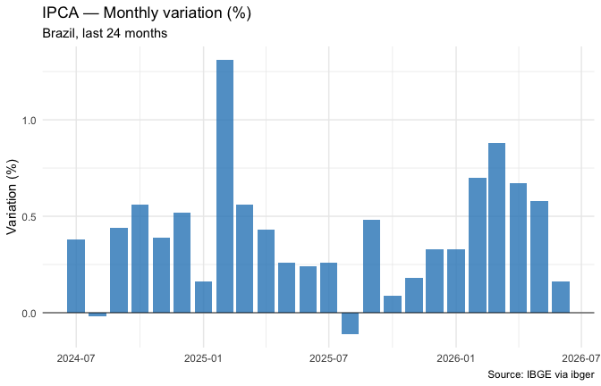
Step 3 — Compare accumulation measures
Get all three variation variables at once:
ipca_vars <- ibge_variables(
  aggregate  = 7060,
  variable   = c(63, 69, 2265),
  periods    = -12,
  localities = "BR"
)

ipca_vars <- ipca_vars |>
  mutate(
    value = parse_ibge_value(value),
    date  = as.Date(paste0(period, "01"), format = "%Y%m%d")
  )

ggplot(ipca_vars, aes(date, value, colour = variable_name)) +
  geom_line(linewidth = 0.8) +
  geom_point(size = 1.5) +
  labs(
    title  = "IPCA — Three measures of variation",
    x = NULL, y = "%", colour = NULL,
    caption = "Source: IBGE via ibger"
  ) +
  theme_minimal() +
  theme(legend.position = "bottom")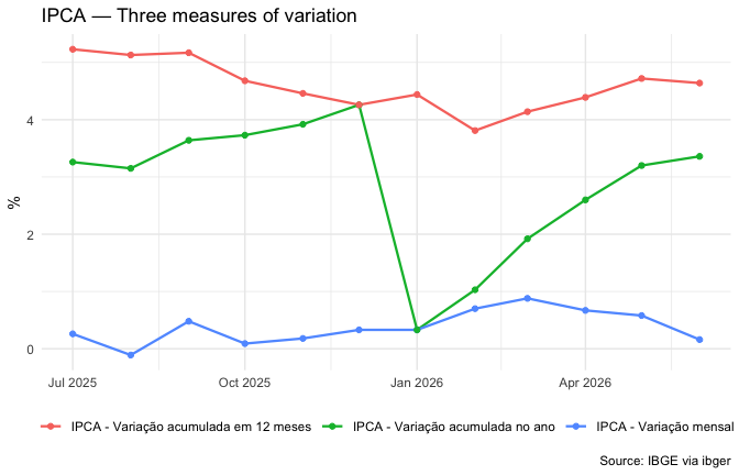
Step 4 — Breakdown by product group
Classification 315 organizes IPCA items hierarchically. The top-level groups (level 1 categories) are things like Food and beverages (7170), Housing (7445), Transportation (7486), etc.
First, find the category IDs you need:
cats <- tidyr::unnest(meta$classifications, categories)

# Level-1 groups (just below the general index)
cats |> filter(category_level == "1")
#> # A tibble: 9 × 6
#>   id    name              category_id category_name category_unit category_level
#>   <chr> <chr>             <chr>       <chr>         <chr>         <chr>
#> 1 315   Geral, grupo, su… 7170        1.Alimentaçã… <NA>          1
#> 2 315   Geral, grupo, su… 7445        2.Habitação   <NA>          1
#> 3 315   Geral, grupo, su… 7486        3.Artigos de… <NA>          1
#> 4 315   Geral, grupo, su… 7558        4.Vestuário   <NA>          1
#> 5 315   Geral, grupo, su… 7625        5.Transportes <NA>          1
#> 6 315   Geral, grupo, su… 7660        6.Saúde e cu… <NA>          1
#> 7 315   Geral, grupo, su… 7712        7.Despesas p… <NA>          1
#> 8 315   Geral, grupo, su… 7766        8.Educação    <NA>          1
#> 9 315   Geral, grupo, su… 7786        9.Comunicação <NA>          1
Now query specific groups:
groups <- ibge_variables(
  aggregate      = 7060,
  variable       = 63,
  periods        = -12,
  localities     = "BR",
  classification = list("315" = c(7170, 7445, 7486, 7558, 7625, 7660, 7712, 7766, 7786))
)

groups <- groups |>
  mutate(
    value = parse_ibge_value(value),
    date  = as.Date(paste0(period, "01"), format = "%Y%m%d")
  )

ggplot(groups, aes(date, value, fill = classification_315)) +
  geom_col(position = "dodge", alpha = 0.85) +
  labs(
    title = "IPCA by product group — Monthly variation",
    x = NULL, y = "%", fill = NULL,
    caption = "Source: IBGE via ibger"
  ) +
  theme_minimal() +
  theme(legend.position = "bottom", legend.text = element_text(size = 7))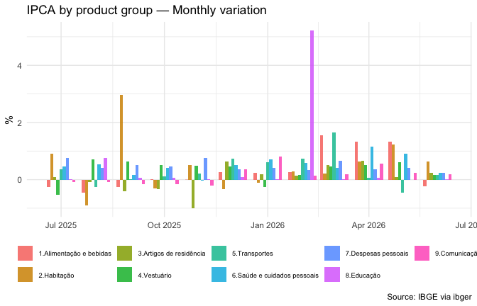
Step 5 — Metropolitan area comparison
Aggregate 7060 is available at level N7 (metropolitan areas). Compare inflation across major cities:
# Check available metropolitan areas
metros <- ibge_localities(7060, level = "N7")
metros
#> # A tibble: 0 × 4
#> # ℹ 4 variables: id <chr>, name <chr>, level_id <chr>, level_name <chr>
Pick a few and compare:
ipca_metros <- ibge_variables(
  aggregate  = 7060,
  variable   = 2265,
  periods    = -12,
  localities = list(N7 = c(3501, 3301, 2901, 4101, 1501))
)

ipca_metros <- ipca_metros |>
  mutate(
    value = parse_ibge_value(value),
    date  = as.Date(paste0(period, "01"), format = "%Y%m%d")
  )

ggplot(ipca_metros, aes(date, value, colour = locality_name)) +
  geom_line(linewidth = 0.8) +
  labs(
    title   = "IPCA — 12-month cumulative by metro area",
    x = NULL, y = "%", colour = NULL,
    caption = "Source: IBGE via ibger"
  ) +
  theme_minimal() +
  theme(legend.position = "bottom")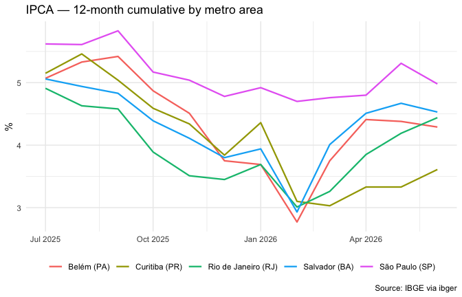
Step 6 — Building a complete dataset
For a more complete analysis, combine multiple queries. For instance, download the general index for all metro areas and reshape:
all_metros <- ibge_variables(
aggregate = 7060,
variable = c(63, 69, 2265),
periods = -12,
localities = "N7",
classification = list("315" = 7169)
)
all_metros <- all_metros |>
mutate(value = parse_ibge_value(value)) |>
select(variable_name, locality_name, period, value) |>
pivot_wider(names_from = variable_name, values_from = value)
all_metros
#> # A tibble: 120 × 5
#> locality_name period `IPCA - Variação mensal` IPCA - Variação acumulada no …¹
#> <chr> <chr> <dbl> <dbl>
#> 1 Belém - PA 202509 0.27 3.47
#> 2 Belém - PA 202510 0.26 3.74
#> 3 Belém - PA 202511 0.11 3.85
#> 4 Belém - PA 202512 -0.1 3.75
#> 5 Belém - PA 202601 0.16 0.16
#> 6 Belém - PA 202602 0.62 0.78
#> 7 Belém - PA 202603 1.31 2.11
#> 8 Belém - PA 202604 1.08 3.21
#> 9 Belém - PA 202605 0.63 3.86
#> 10 Belém - PA 202606 0.07 3.93
#> # ℹ 110 more rows
#> # ℹ abbreviated name: ¹`IPCA - Variação acumulada no ano`
#> # ℹ 1 more variable: `IPCA - Variação acumulada em 12 meses` <dbl>Large queries
IPCA has several hundred categories in classification 315. Querying
all of them for many periods and every metro area quickly exceeds the
API’s per-request limit. You do not have to split such a query yourself:
ibge_variables() estimates the result size and, when
needed, splits the request (by periods, then by localities) and binds
the pieces back together — see the chunk argument in
?ibge_variables. The full breakdown for one period and
Brazil fits in a single request:
full_breakdown <- ibge_variables(
  aggregate      = 7060,
  variable       = 63,
  periods        = -1,
  localities     = "BR",
  classification = list("315" = "all")
)

nrow(full_breakdown)
#> [1] 457
Even with automatic splitting, narrowing the periods, localities or categories to what you actually need keeps the queries fast: the IBGE API takes noticeably longer to answer large requests.
Handling special values
The value column returned by
ibge_variables() is always character, because the IBGE API
uses special codes for certain data conditions. Use
parse_ibge_value() to convert to numeric in one step:
ibge_variables(7060, localities = "BR") |>
  mutate(value = parse_ibge_value(value))
#> # A tibble: 24 × 9
#>    variable_id variable_name        variable_unit classification_315 locality_id
#>    <chr>       <chr>                <chr>         <chr>              <chr>
#>  1 63          IPCA - Variação men… %             Índice geral       1
#>  2 63          IPCA - Variação men… %             Índice geral       1
#>  3 63          IPCA - Variação men… %             Índice geral       1
#>  4 63          IPCA - Variação men… %             Índice geral       1
#>  5 63          IPCA - Variação men… %             Índice geral       1
#>  6 63          IPCA - Variação men… %             Índice geral       1
#>  7 69          IPCA - Variação acu… %             Índice geral       1
#>  8 69          IPCA - Variação acu… %             Índice geral       1
#>  9 69          IPCA - Variação acu… %             Índice geral       1
#> 10 69          IPCA - Variação acu… %             Índice geral       1
#> # ℹ 14 more rows
#> # ℹ 4 more variables: locality_name <chr>, locality_level <chr>, period <chr>,
#> #   value <dbl>
The function handles all IBGE conventions — "-" becomes
0 and the “not available” codes become NA. See
?parse_ibge_value for the full table of codes and their
meanings.
parse_ibge_value(c("1.5", "10", "-", "..", "...", "X"))
#> [1]  1.5 10.0  0.0   NA   NA   NA